 Stratum
Correlation vs Causation: Pearson vs Spearman
Correlation measures how two variables move together — but it doesn't tell you why. And there's more than one way to measure it. Here's what you actually need to know.
A correlation coefficient runs from −1 to +1: near +1 the two variables rise together, near −1 one rises as the other falls, near 0 there's no linear relationship. Simple — but two cautions trip people up.
Two ways to measure: linear vs rank
Pearson's r measures linear association — how tightly the points hug a straight line — from the raw values, so one extreme point can swing it hard. Spearman's ρ and Kendall's τ throw the raw values away and work on the ranks (1st, 2nd, 3rd…). That makes them measure any monotonic relationship — consistently up or down, even if it curves — and shrug off outliers. When Pearson and the rank measures disagree, the gap is the finding. Here are the two cases where they part ways.
Case 1 — a perfect climb that isn't a straight line
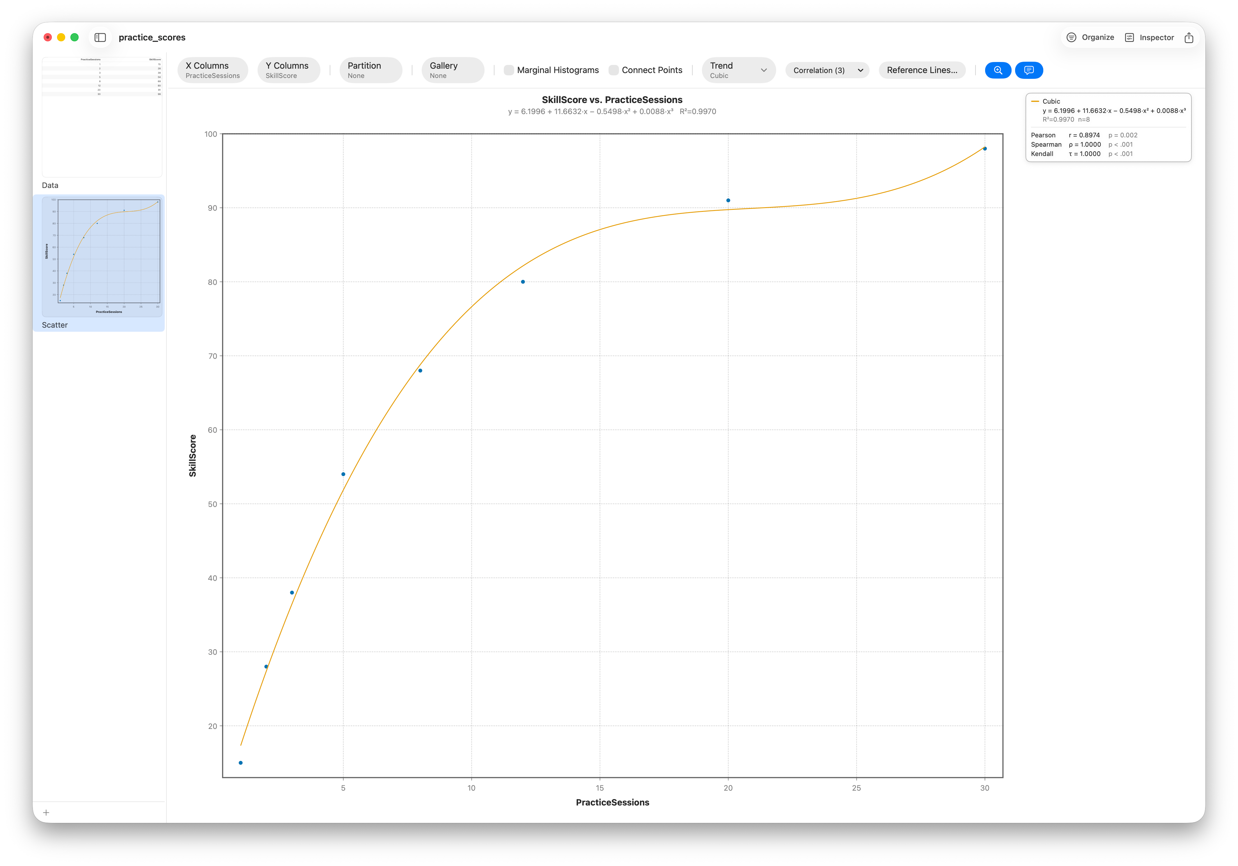
Practice sessions versus a skill score. Every session helps, but with diminishing returns — the classic learning curve:
| Practice sessions | Skill score |
|---|---|
| 1 | 15 |
| 2 | 28 |
| 3 | 38 |
| 5 | 54 |
| 8 | 68 |
| 12 | 80 |
| 20 | 91 |
| 30 | 98 |
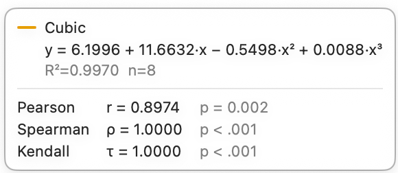
The ranking is flawless — more practice always means a higher score — so Spearman ρ = 1.00 and Kendall τ = 1.00. But the climb bends, so Pearson r = 0.90. Pearson isn't wrong; it's answering a narrower question ("how straight-line?") than the one you usually care about ("do they move together?"). Trust Pearson alone here and you'd under-rate a rock-solid relationship. Grab the data — practice_scores.csv — and try it.
Case 2 — one outlier that invents a correlation
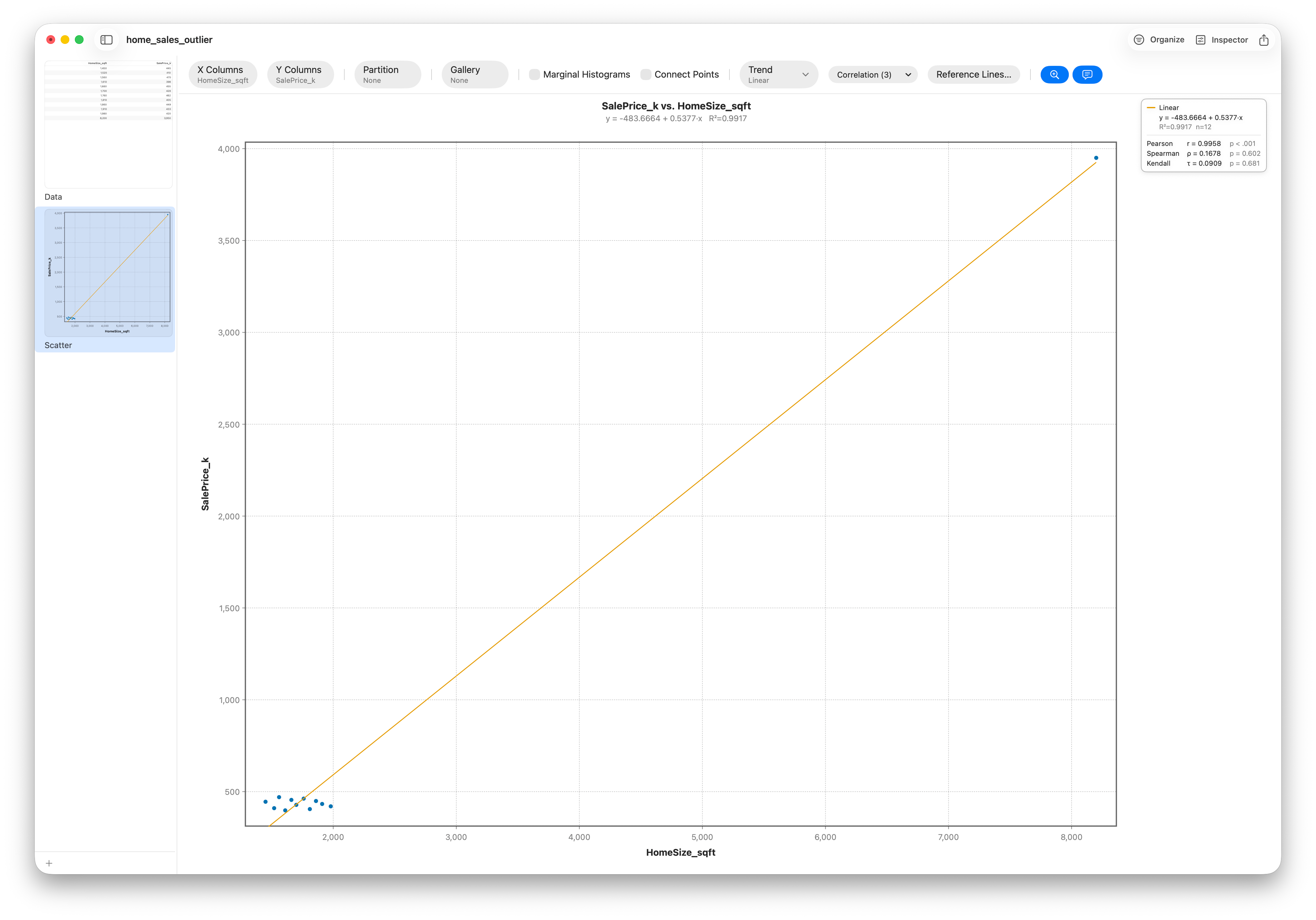
Twelve home sales in one neighborhood. Eleven are ordinary mid-size houses; the twelfth is a mansion:
| Home size (sq ft) | Sale price ($k) |
|---|---|
| 1,450 | 445 |
| 1,520 | 410 |
| 1,560 | 470 |
| 1,610 | 398 |
| 1,660 | 455 |
| 1,700 | 428 |
| 1,760 | 462 |
| 1,810 | 405 |
| 1,860 | 449 |
| 1,910 | 433 |
| 1,980 | 420 |
| 8,200 | 3,950 |
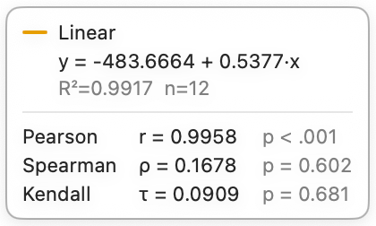
Among the eleven ordinary homes, size barely tracks price: Pearson r = −0.11 — essentially nothing. Add the single mansion and Pearson leaps to 0.996, screaming "near-perfect correlation." It's a mirage. The rank measures aren't fooled: Spearman ρ = 0.17 and Kendall τ = 0.09, still basically zero. The whole "correlation" rests on one high-leverage point — drop the mansion and it evaporates. Grab the data — home_sales_outlier.csv.
What about Kendall's τ?
Kendall's τ is the other rank-based coefficient. Rather than correlating the ranks like Spearman, it counts concordant versus discordant pairs — for every two rows, do both variables agree on which is larger? Being rank-based, it tells the same story as Spearman (note ρ = τ = 1.00 in Case 1, and both near zero in Case 2). It usually runs a little smaller in magnitude, and it's the steadier choice for small samples or data with many tied values. Use Spearman when you want something on Pearson's familiar −1-to-+1 scale; reach for Kendall when you want the most robust, easy-to-defend number.
The trap: correlation isn't causation
Even a real, well-measured correlation doesn't tell you why. Two variables can move together because one causes the other, because a third factor drives both, or by sheer coincidence. Ice-cream sales correlate with drownings — not because cones are dangerous, but because hot weather drives both. A correlation is a starting point for a question, never the answer to it.
In Stratum
Every coefficient above came straight from Stratum. On any scatter, switch on Correlation in the control bar to print Pearson, Spearman and/or Kendall — each with its p-value — right on the plot, exactly as in the figures here. Prefer a table? The Correlation analysis shows one method at a time, with a Method switch to compare them. Grab practice_scores.csv and home_sales_outlier.csv and see both cases for yourself.
Frequently asked questions
When should I use Spearman instead of Pearson?
Use Spearman when the relationship is monotonic but curved, when the data is skewed, or when outliers would distort Pearson's r. Spearman works on ranks, so it's more robust.
Does correlation imply causation?
No. A strong correlation means two variables move together; it doesn't say one causes the other. A lurking third variable or coincidence can produce the same pattern.
What is a strong correlation?
Loosely, |r| above ~0.7 is strong, ~0.3–0.7 moderate, below ~0.3 weak — but always read it alongside a scatter plot and your sample size.
Can two variables be related but have zero correlation?
Yes — correlation only measures linear (Pearson) or monotonic (Spearman) association. A U-shaped relationship can have near-zero correlation while being perfectly real.
What’s the difference between Spearman and Kendall?
Both are rank-based, so they usually agree. Spearman correlates the ranks and shares Pearson’s −1-to-+1 scale; Kendall counts concordant vs discordant pairs, tends to run smaller in magnitude, and holds up better with small samples or many ties. Stratum offers both — you flip the Method switch to see each.